Quantcast
Channel: Statalist
Viewing all 65472 articles
Browse latest View live

Estimating the significance of fixed effects with clustered standard errors

$
0
0
Hi all,

I am estimating the following equation.

Code:
 xtreg lemp lunion lunemployment lfertility lyouth i.year, fe vce(cluster id)
.

I am interested in calculating the significance of the fixed effects. However, since I am clustering my data u_i = 0 no longer appears.

I have tried estimating the equation as:

Code:
 reg lemp lunion lunemployment lfertility lyouth i.year i.id, vce(cluster id)
.

Then conducting a Wald test:

Code:
 testparm i.id
However, I am obtaining some very high estimates, some over 40,000, so I am not sure I am calculating this correctly.

I would really appreciate any help with this - whether I am computing this incorrectly, or if there is some other issue causing my F-statistics to be so large.

Thank you.

Calculating adjusted proportions

$
0
0
There are examples of analyses using Stata (14) that calculates proportion of one variable by adjusting for another (e.g. age-adjusted prevalence of diabetes), but this option is nowhere to be found within Stata. Is there any user written command for this? Array

graph with a small line?

$
0
0
Dear All, I have this graph
Array
by the following data and code.
Code:
* Example generated by -dataex-. To install: ssc install dataex
clear
input float(growth lprivo) str3 code
  .6176451  2.752746 "ARG"
 1.9751474  4.004016 "AUS"
  2.889185  4.178968 "AUT"
  .7082631 2.6060796 "BGD"
  2.652859  3.704847 "BRB"
 2.6513345 3.2444575 "BEL"
  .3550578 2.5758026 "BOL"
 2.9300966  3.065546 "BRA"
 2.3859885 4.1086454 "CAN"
 1.4469954   3.32541 "CHL"
 2.2270143  3.094773 "COL"
 1.6136966 3.0807066 "CRI"
  5.384184  4.127378 "CYP"
 2.1793702  3.748256 "DNK"
  2.498769 2.9503646 "DOM"
  2.388093  2.889542 "ECU"
 -.6075561 3.1289306 "SLV"
 1.8458964  3.163393 "FJI"
  2.798494  3.947039 "FIN"
  2.431281  4.323712 "FRA"
  2.453688  4.336713 "DEU"
 -.9631622 1.6240644 "GHA"
   3.22405   3.60341 "GRC"
  .9292306  2.589061 "GTM"
-.28062087  3.021234 "GUY"
 -.6579341  2.042972 "HTI"
  .5977848 3.1720316 "HND"
  3.012389 3.5494244 "ISL"
  1.915168 2.9719946 "IND"
  3.254494 3.8947036 "IRL"
  2.810969  3.622525 "ISR"
 2.9329815 4.0790596 "ITA"
  .4177902  3.200545 "JAM"
  4.304759  4.854981 "JPN"
  1.962509 3.1259286 "KEN"
  7.156855 4.1817265 "KOR"
 -.4721583  2.318493 "LBR"
  4.114544 3.8480165 "MYS"
  6.652838 3.7835095 "MLT"
  3.024178 3.1929696 "MUS"
 1.9739418  3.130883 "MEX"
  .7671511  2.044247 "NPL"
 2.2005773 4.4623857 "NLD"
 1.1241318  3.626801 "NZL"
 -2.751478  2.568801 "NER"
  3.182494  4.402111 "NOR"
  2.698163 3.0333946 "PAK"
 2.0271885  3.694385 "PAN"
 1.1203711  3.037085 "PNG"
 2.3819315 2.6755195 "PRY"
 .06020596  2.589619 "PER"
 1.1587406 3.2949524 "PHL"
   3.64731 4.0075636 "PRT"
 -.4378241 3.3143885 "SEN"
 -.3398342 1.6226246 "SLE"
  .3920211  4.275775 "ZAF"
  2.880327  4.175143 "ESP"
 2.7045984 2.7856154 "LKA"
 1.8881342 4.4898977 "SWE"
 1.4218653  4.950846 "CHE"
  2.511772 2.1776114 "SYR"
  6.624734  4.057945 "TWN"
  4.876695  3.856032 "THA"
  .4627753 3.0857854 "TGO"
 1.1207864 3.4465425 "TTO"
 1.9622195  3.835404 "GBR"
  1.712265   4.72797 "USA"
 1.0253086 3.0545275 "URY"
 -.8835508  3.500184 "VEN"
-2.8119445 1.4072825 "ZAR"
  .8381555  3.137074 "ZWE"
end

twoway (scatter growth lprivo, mlabel(code) ms(oh)) (lfit growth lprivo), ytitle(growth) legend(off)
I'd like to have a short line (for example, Netherlands, France, Portugal) like the following graph (Note that the data sets are different).
Array
Any suggestions? Thanks.

use of difference in unbalanced panel data

$
0
0
I am having unbalanced panel data of 84 countries, now the objective of my empirical investigation will be done if i convert my dependent variable into log.difference(growth rate). when i do so results for my independent and control variables turns insignificant. and when i apply difference on control and independent variable the results become significant and according to theory.
I wonder if taking difference is appropriate with unbalanced structures? and why the difference need to be applied on rest of the variables too.

Margins different between male and female?

$
0
0
Clyde Schechter

I ran this regression equation

Code:
reg income c.age i.educ i.sex c.workhours
where wageincome is income ,

educ is in 3 categories (1) not less of education (2) some level of education (3) degree and above

and workhours is hours worked.

sex = 0 and 1 for male, female respectively.

predicted probabilities


Code:
margins, at( sex=(0) educ=(3) workhours=(20(20)80)) vsquish
Code:
margins, at( sex=(1) educ=(3) workhours=(20(20)80)) vsquish

what will be the different between male and female?

import many csv files

$
0
0
Dear All, I generate many csv and excel files as
Code:
cd "E:\Stata\import data\manycsv"

webuse grunfeld, clear

preserve
keep if company == 1
export excel using "a1.xls", firstrow(variables) replace
export delimited using "a1.csv", replace
restore

preserve
keep if company == 2
export excel using "b2.xls", firstrow(variables) replace
export delimited using "b2.csv", replace
restore

preserve
keep if company == 3
export excel using "c3.xls", firstrow(variables) replace
export delimited using "c3.csv", replace
restore
I tried to follow the thread (https://www.statalist.org/forums/for...many-csv-files) to import those generated csv files as
Code:
// ssc inst fs 
clear
cd "E:\Stata\import data\manycsv"
fs *.csv 
foreach f in `r(files)' {   
  insheet using "`f'", clear 
  *local ID: subinstr local f "NYSE_" "", all 
  save "`f'.dta", replace
}
I have "a1.csv.dta, b2.csv.dta, and c3.csv.dta. How can I modify the code to get resulting files as a1.dta, b2.dta, and c3.dta? Thanks.

Data manipulation for ciplot

$
0
0
I use -ciplot- to show the state of Health (1Very Good...5Very bad) across Age. -ciplot- graphs the mean values of Health but I want to plot it as count (1,2,3,4,5) instead. Is there any way to trick the process e.g. transforming the data structure.

Code:
* Example generated by -dataex-. To install: ssc install dataex
clear
input double(Age Health)
85 4
40 2
73 2
50 3
51 2
62 3
43 2
69 2
27 3
55 4
59 3
50 2
72 4
75 3
31 2
53 3
65 3
44 3
72 3
64 2
54 2
65 2
70 2
59 3
50 2
54 4
70 2
73 3
54 3
38 1
79 2
50 2
57 3
46 2
53 4
85 4
79 3
31 2
50 4
35 2
61 2
70 3
50 2
37 2
87 3
54 2
62 3
50 3
55 3
50 2
62 2
60 2
61 3
52 1
70 2
70 3
60 3
72 3
64 3
61 3
67 3
74 3
56 3
80 2
52 2
90 4
50 3
66 4
67 4
46 3
86 4
57 3
70 2
65 3
56 4
74 3
65 3
55 2
71 2
62 3
60 3
52 3
78 3
55 2
81 4
37 1
52 3
55 3
75 4
38 2
50 2
73 3
28 1
64 2
75 4
82 3
68 3
75 2
50 3
49 2
end
Code:
ciplot Health, by(Age)
Array

reshape or what?

$
0
0
Dear All, I have this dataset,
Code:
* Example generated by -dataex-. To install: ssc install dataex
clear
input str3 code str4 seriesname double(yr2015 yr2016 yr2017)
"CAN" "inf"    1.12524136094279    1.4287595470108    1.5968841285297
"JPN" "inf"    .789517890139427  -.116666666666671   .467211747038214
"USA" "inf"    .118627135552435   1.26158320570537   2.13011000365963
"CAN" "prvt"                  .                  .                  .
"JPN" "prvt" 162.30694503499905 162.35440967317416 168.19138836880097
"USA" "prvt"  188.2037313190976  192.1654998496473                  .
end
and wish to have the following result
Code:
* Example generated by -dataex-. To install: ssc install dataex
clear
input str3 code double(inf2015 inf2016 inf2017) double(prvt2015 prvt2016 prvt2017)
"CAN"   1.12524136094279    1.4287595470108    1.5968841285297                   .                  .                  .
"JPN"   .789517890139427  -.116666666666671   .467211747038214  162.30694503499905 162.35440967317416 168.19138836880097
"USA"   .118627135552435   1.26158320570537   2.13011000365963   188.2037313190976  192.1654998496473                  .
end
Any suggestions are appreciated!

Graph bar with custom labels

$
0
0
Dear Statalist

I have been struggling with the following issue for quite a while now. Unfortunately I am not able to display any dataex as my data is found on a remote desktop at my workplace. Hopefully my description will make do - my apologies!

And a disclaimer: my issue relates to this question https://www.statalist.org/forums/for...s-in-bar-graph, but I have not been able to grasp exactly how I should approach it though, so therefore I took myself the liberty of asking in a new thread.

Description of my situation
I have population data on 0 to 24 year olds. Furthermore, I have three relevant variables: one displaying which age-bracket the individual belongs to (0-4; 5-9; 10-14; 15-19; 20-24) and another categorical variable displaying which of 11 specific illnesses - if any - an individual might have had. An individual might appear more than once (and app. 50% do that) if they have had two or more illnesses. Lastly, I have a variable indicating the individuals gender. All three variables are strings at the moment but can be changed accordingly.

I am trying to create 11 bar graphs - one for each illness - with the percentage of each sub-group who have had the specific illness on the Y-axis, split into both age-brackets and gender on the X-axis. So for example: the first two bars should reflect the percentage of 0-4 year old boys and girls, respectively, who have had the illness. The next two bars should reflect the percentage of 5-9 year old boys and girls with the same illness, etc. To be more exact: my population consists of almost 2,5 million unique id's but due to the possibility of reappearing, my dataset is almost 4,0 million observations. The aforementioned percentage should only reflect the share of unique individuals.

As labels, I would like to have the number of individuals who have had the illness and this is where I run into trouble. I am able to create the graphs using -graph bar-, but it is not possible to use N as custom labels. In the aforementioned former question on Statalist, it is argued that -collapse- and -twoway- can be used. If that is applicable in my situation as well, I could really use a description of how to approach it.

Thany you!

SOEP weighting

$
0
0
Hi,
I am new to STATA and have a project where I use SOEP data. I would like to calculate a weighted mean savings rate and therefore have to weight the net income per month and savings per month. How do I weight them with the given weights and calculate then the mean ?

Thank you very much in advance!
Fabian

How to generate 2 yaxis graph with 2 xaxis group with SD?

$
0
0
I have the information here, on the table
weeks ISpre A1M B2M sdis sdam sdbm group hiISpre loISpre hiB2M loBM hiA1M loA1M
1 4 2 46 3 1 11 2 5 2 53 39 3 1
2 3 3 41 2 1 9 2 5 2 46 35 3 2
3 2 2 42 2 1 8 2 3 1 47 37 3 2
1 4 3 50 3 1 16 1 5 2 60 40 4 3
2 2 3 42 1 1 9 1 3 2 48 36 3 2
3 3 2 41 1 1 10 1 4 2 47 35 3 2
I want to made graph in the figure
I use command
** graph bar b2m A1M ISpre, over(week) over(group) asyvars

but I cannot add SD of the graph (hi and lo) and cannot make twoway command

Could you please to help me?

Thank you

Restrictions on Structural VAR Impulse Response Functions

$
0
0
Dear all,

I would like to impose some restrictions on an estimated SVAR before running impulse response function, by following the work by Ludvigson et al. (2002, Monetary Policy Transmission through the Consumption-Wealth Channel. FRBNY Economic Policy Review,117-133.)

I am using Stata 15.1 for Windows.

By following this tutorial and using the dataset, I have estimated a Structural VAR:

Ayt = C1yt-1 + C2yt-2 ... Ckyt-k + But

Code:
use usmacro.dta

matrix A1 = (1,0,0 \ .,1,0 \ .,.,1)

matrix B1 = (.,0,0 \ 0,.,0 \ 0,0,.)

svar inflation unrate ffr, lags(1/6) aeq(A1) beq(B1)
Estimating short-run parameters

Iteration 0:   log likelihood = -708.74354  
Iteration 1:   log likelihood = -443.10177  
Iteration 2:   log likelihood = -354.17943  
Iteration 3:   log likelihood = -303.90081  
Iteration 4:   log likelihood =  -299.0338  
Iteration 5:   log likelihood = -298.87521  
Iteration 6:   log likelihood = -298.87514  
Iteration 7:   log likelihood = -298.87514  

Structural vector autoregression

 ( 1)  [a_1_1]_cons = 1
 ( 2)  [a_1_2]_cons = 0
 ( 3)  [a_1_3]_cons = 0
 ( 4)  [a_2_2]_cons = 1
 ( 5)  [a_2_3]_cons = 0
 ( 6)  [a_3_3]_cons = 1
 ( 7)  [b_1_2]_cons = 0
 ( 8)  [b_1_3]_cons = 0
 ( 9)  [b_2_1]_cons = 0
 (10)  [b_2_3]_cons = 0
 (11)  [b_3_1]_cons = 0
 (12)  [b_3_2]_cons = 0

Sample:  39 - 236                               Number of obs     =        198
Exactly identified model                        Log likelihood    =  -298.8751

------------------------------------------------------------------------------
             |      Coef.   Std. Err.      z    P>|z|     [95% Conf. Interval]
-------------+----------------------------------------------------------------
      /a_1_1 |          1  (constrained)
      /a_2_1 |   .0348406   .0416245     0.84   0.403     -.046742    .1164232
      /a_3_1 |  -.3777114    .113989    -3.31   0.001    -.6011257   -.1542971
      /a_1_2 |          0  (constrained)
      /a_2_2 |          1  (constrained)
      /a_3_2 |   1.402087   .1942736     7.22   0.000     1.021318    1.782857
      /a_1_3 |          0  (constrained)
      /a_2_3 |          0  (constrained)
      /a_3_3 |          1  (constrained)
-------------+----------------------------------------------------------------
      /b_1_1 |   .4088627   .0205461    19.90   0.000     .3685931    .4491324
      /b_2_1 |          0  (constrained)
      /b_3_1 |          0  (constrained)
      /b_1_2 |          0  (constrained)
      /b_2_2 |   .2394747   .0120341    19.90   0.000     .2158884     .263061
      /b_3_2 |          0  (constrained)
      /b_1_3 |          0  (constrained)
      /b_2_3 |          0  (constrained)
      /b_3_3 |   .6546452   .0328972    19.90   0.000     .5901679    .7191224
------------------------------------------------------------------------------

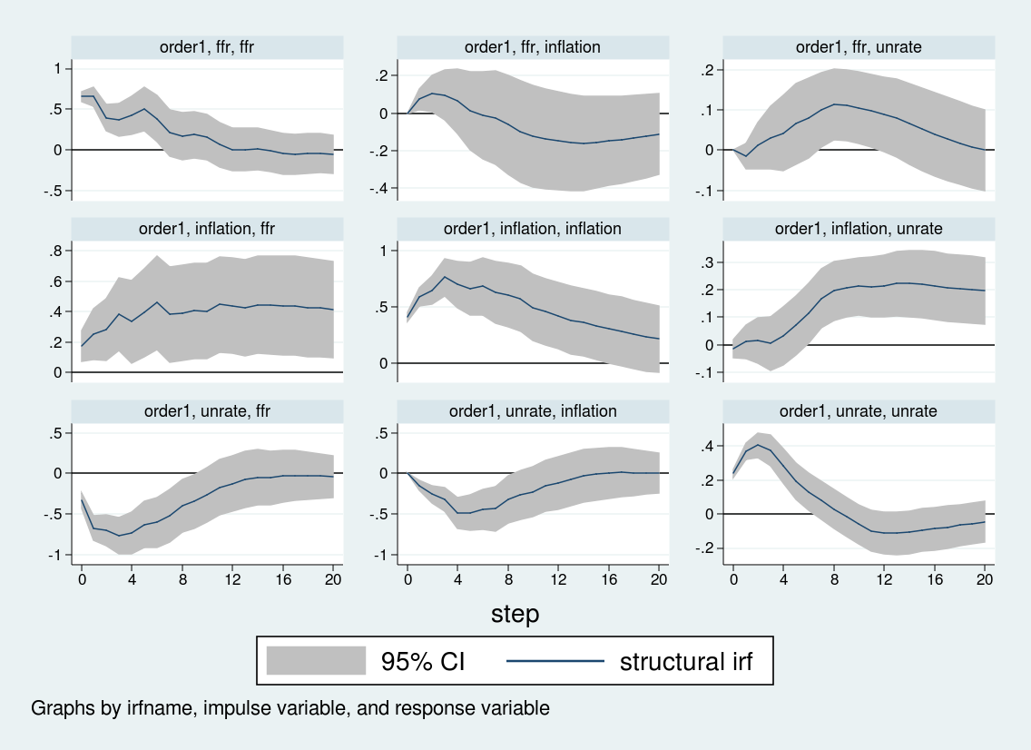
irf create order1, set(var2.irf) replace step(20)

irf graph sirf, xlabel(0(4)20) irf(order1) yline(0,lcolor(black)) byopts(yrescale)
And the figure below shows the impulse response function based on the SVAR estimated above.


Now, I want to perform another impulse response analysis on the estimated Structural VAR by imposing some restrictions on the matrices C0 to Ck. For instance, I want to set c23 = 0 in matrices C0 to Ck to econometrically turn off the effects of the contemporaneous response of the unemployment rate to the federal funds rate, as well as any lagged response of the unemployment rate to the federal funds rate.

Based on this restricted SVAR, I would like to perform impulse response analysis to see the response of inflation rate against a shock in the federal funds rate.
There was a similar discussion about this previously on Statalist, but it seems that no direct solutions were provided.

Is there any way to do this on Stata?
Thank you very much for your help in advance.

Daiki

Unifiying databases

$
0
0
Dear users of StataCorp forum,


As follows I describe my puzzle:


Dataset 1
variables: date cusip prc ret shrout
Dataset 2
variables: fyear cusip bkvlps csho ggroup gsector

The time observations in Dataset 2 are in annual basis, whilst those in Dataset 1 are in monthly basis. Each cusip value corresponds to one unique company and so in Dataset 1 cusip values are repeated for all months when the company´s stock traded.

What I need to do is to set the variables bkvlps csho ggroup gsector from dataset 2, for which I have one observation per year (D2: fyear) and per company (cusip) repeatedly for every month (D1: date) in dataset 1 that belongs to that particular year (D2: fyear) and it must also coincide for that given company (cusip). Therefore, at the end, I should have a unique dataset that has the variables date cusip prc ret shrout bkvlps csho ggroup gsector wherein the variables bkvlps csho ggroup gsector repeat accordingly to cusip and to date depending on whether the month in date coincides with one within the year fyear.


Dataset 1

Array


Dataset 2

Array


In the images you can observe only one cusip, ggroup, and gsector, but the variable cusip changes and is unique for each different firm while the ggroup and gsector remain constant across the time-series for each cusip but are not unique to that particular company as is the cusip.


If you need any more information to help me with this puzzle, do not hesitate in asking me.

Thank you for your time and attention.

How to compare β coefficients from two different logistic regression models using permutation test

$
0
0
Hi everyone,

I am running two logistic regression models, in which only dependent variables are different and all the 6 independent variables are same.
I just want to know whether one of the β coefficients from one model is larger than that from the other model using permutation test instead of using suest/Hausman specification test.
However, I had completely no idea how to type command to complete this task on Stata.

I would really appreciate any help I might get here.

Yuki Ishikawa

Panel Var

$
0
0
dear all,
i have stata 13 and i'm trying to do panel var. i've cleaned the data, but whenever i try to start using pvar pachage, it doesn't work, the command just keep operating for hours without giving results or even give error
can you help me figuring out what is the problem

Drop command

$
0
0
Clyde Schechter

I will like will to create a database from an existing data for only individuals aged 16 - 65 who are employed, in labor force, have income above zero and working hours above zero or missing.

I have three variables empstat, labfroce,incwage, uhrswork

empstat which has a category for (1) N/a (2) employed (3) Unemployed and (4) Not in labor force.

labforce which has category for (1) N/A (2) No, Not in the labor force and (3) in the labor force.

will the following codes be right?

Code:
drop if age <16
Code:
drop if age >65

Code:
drop if empstat ==2| age <16
Code:
drop if empstat ==2| age >65
Code:
drop if empstat==0| age <16

Code:
drop if empstat==0| age >65


Code:
drop if empstat==3| age <16
Code:
drop if empstat==3| age >65
*Dropping labour force data

Code:
drop if labforce ==1| age <16
Code:
drop if labforce ==1| age >65


Code:
drop if incwage ==0 |age <16
Code:
drop if incwage ==0 |age >65
Code:
drop if uhrswork==0 |age <16
Code:
drop if uhrswork==0 |age >65

Clyde Schechter

Fixed Effects and Random Effects

$
0
0
Hi Dear,

Can you please tell me whether Fixed Effects estimations with xtreg, fe and Random Effects estimations with xtreg, re produce long run or short run estimates?

Thank you.

recode two continuous variables into one categorical(3 categories) variable

$
0
0
I am new to Stata and I am trying to recode two continuous variables into one categorical(3 categories) variable. I pasted data from dataex below. The continuous variables are "vigmin" and "modmin"(see definition below).

Vigmin = the number minutes someone participated in vigorous activity in a week

Modmin = the number minutes someone participated in moderate activity in a week

“.” = the period is treated as 0 minutes of activity, so any “.” should equal “poor(3).

Desired categories for the new categorical variable:

Ideal(1) = 150 minutes or greater of moderate physical activity per week, or 75 minutes or greater of vigorous activity per week

Intermediate(2) = 1 – 149 minutes of moderate physical activity per week, or 1 - 74 minutes of vigorous activity per week

Poor(3) = 0 minutes of activity


This is the syntax that I tried; I did not get an error, but the numbers in my output were not accurate. Should I be using different syntax?
gen idealPA=0
replace idealPA=1 if (modmin >=150) | (vigmin >=75)
replace idealPA=2 if (modmin >=1) & (modmin <=149)
replace idealPA=2 if (vigmin >=1) & (vigmin <=74)
replace idealPA=3 if (modmin==.) | (vigmin==.)
label define idealPA 1 "ideal" 2 "intermediate" 3 "Poor"
label value idealPA idealPA
ta idealPA RCTgroup, row col chi


(example data from Dataex)

Code:
* Example generated by -dataex-. To install: ssc install dataex
clear
input float(modmin vigmin)
105  50
  .   .
 60   .
180  30
 20   .
 60   .
 60   .
 30   .
 90   .
  .   .
  .   .
180   .
 60   .
 60   .
180   .
  .   .
 90  20
 60   .
 15  15
 30   .
 60   .
 60   .
120   .
 40   .
 60 180
 45   .
  .   .
 10   .
 90   .
 60  20
 30  35
 40   .
 30  60
 60  30
180 105
 25   .
180  60
 60 120
120  30
120   .
  .  10
120   .
120 120
 40 180
 60  30
180   .
180  20
 60   .
 25   .
180  30
 30   .
 60  60
 30   .
  .   .
150   .
 10 180
  .   .
 20  15
120   .
 30   .
 90  10
180   .
 60   .
 30  30
  .  10
 30   .
 30 180
 30   .
 60   .
 90  90
 60  10
 20  10
 20  15
 45  60
 25   .
180   .
 60 120
120  90
 15   .
 15   .
 15  10
180  60
  .   .
  .   .
 30   .
  .   .
 75   .
  .   .
  .   .
 10   .
 10   .
  .   .
  .   .
  .   .
 20  10
 10   .
  .   .
  .   .
 25   .
  .   .
end


Thanks in advance for any assistance.

Help Needed on Plotting Rates by Categorical variable

$
0
0
Dear Stata Community,


I have three variables: an event_ind (indicating event occurs) and an education indicator and marital indicator. I want to find the rates of the event indicator over different education and marital groups. Effectively there will be 8 groups (4 education and 2 marital) and I want to plot the rates where event_ind=1 across groups.

A sample chart would have eight bars corresponding to each of the groups showing the rates where event_ind=1.
i
Thanks in advance

Code:
input float(event_ind mother_edind marital_ind)
1 4 1
0 2 2
0 2 1
0 3 2
1 3 1
0 3 1
0 2 1
0 3 2
1 3 1
0 2 1
0 3 1
1 2 1
0 3 1
0 2 2
0 2 2
0 4 1
1 2 1
0 2 1
0 2 2
0 3 1
end
label values vlow_wt_ind lbw2
label def lbw2 0 "Event:0", modify
label def lbw2 1 "Event:1", modify
label values mother_edind edu
label def edu 1 "<High School", modify
label def edu 2 "High School/GED", modify
label def edu 3 "College", modify
label def edu 4 "College+", modify
label values marital_ind mar
label def mar 1 "Married", modify
label def mar 2 "Single", modify

conformability error (503) in Synthetic control method

$
0
0
I am facing the issue of “conformability error (503)” while running the synth command in Stata 15.1.
My data looks like below

Dis qtr od fem_hd poor rural
101 176 .6428571 .0714286 0 .6428571
101 186 .7058824 .1176471 .1764706 .7058824
105 162 1 1 0 1
105 184 .4 .4 0 .8
110 180 .4285714 0 0 .7857143
205 168 .75 0 .25 1
205 176 .7407407 .0185185 .0925926 .3888889
600 187 .7482759 .0396552 .2948276 .7775862

qtr (min 152- max 221) is time variable and Dis is the Panel variable

tsset dis qtr
(it is unbalanced data with gaps)

I run the following command

synth od fem_hd poor rural, trunit(600) trperiod(174)
and it give conformability error 503

I have tried the synth2 version correcting the do file at line 3 and 672 and then synth_wrapper do file at 35

synth2 od fem_hd poor rural, trunit(600) trperiod(174)
but it give the same error.

Ashar
Viewing all 65472 articles
Browse latest View live


<script src="https://jsc.adskeeper.com/r/s/rssing.com.1596347.js" async> </script>